*=============Handling_LapTop_Waveforms=====================
Laptops contain resources to power up a circuit and monitor waveforms.
Many free applications can display the waveforms like an oscilloscope.
The X/Y plot feature can display waveforms like curve tracers.
But Curve tracers plots should be in units like volts and amps.
*=============How_to_Translate=====================
Translation requires some free open source software.
One application can capture the waveforms.
The other application handles offset and gain errors.
And it can display the waveform properly.
But some calibration of the laptop hardware is also required.
*=============The_Audio_Hardware=====================
Laptops will have a stereo input which can capture audio signals.
The coupling is AC with the low frequency 3dB point being around 20Hz.
This input is not intended to handle signals in the voltage magnitude.
A 1meg series resistor at the inputs will extend the range.
A 1meg resistor allows a MacBook Pro to handle about +/-8volts.
Quad RRIO op amps typically are able to swing pretty close to both rails.
One can almost eyeball the input range.
*=============Capture_With_Audacity=====================

Open source software like Audacity can capture waveforms.
The maximum magnitude is +/- one.
A digital +/- one may not represent a standard input voltage.
But calibrating the input of a laptop can be done to some precision.
*=============Capture_and_Trim_A_Waveform=====================
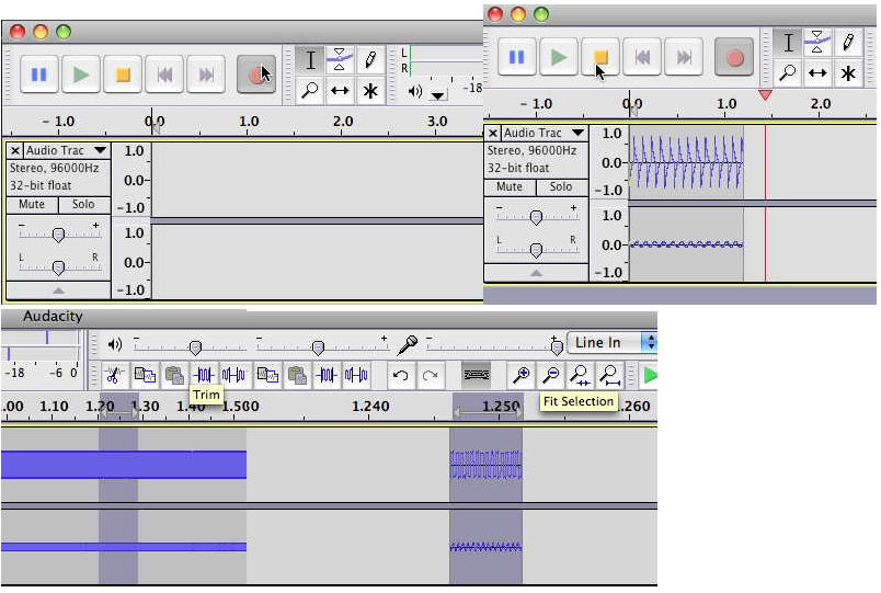
One can capture and trim waveforms very well.
Eye balling the magnitude might needs some improvement.
*=============Save_the_Capture_Waveform=====================
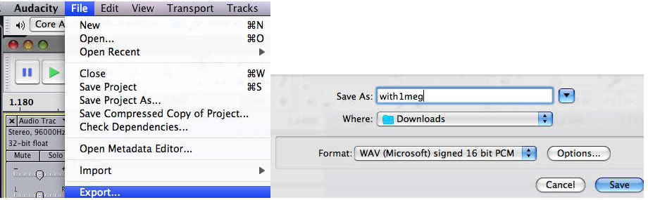
The captured waveform can be exported.
Another free open source application can get a more precise look at the waveform.
For this example, a rail to rail 5Volt output waveform has been captured.
*=============SciLab_Adjusts_Offset_and_Gain=====================

This scilab software provides a better way to handle the waveforms.
The application is run by pasting text into a scilab window.
Scilab will then do all the work.
*=============Find_the_Path=====================
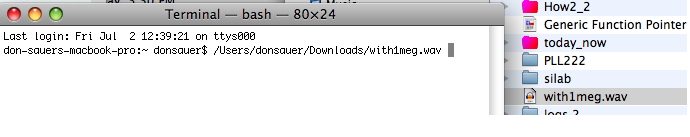
But first hopefully one knows how to find a path to a file.
On a MacBookPro, simply drag and drop a file into a terminal window.
*=============Using_Scilab=====================
After installing Scilab, download this file.
Find its path.
Copy and paste the text below into a text editor.
It should be possible to copy the text from a pdf file or a web page.
Then correct the file path.
Copy and paste the corrected text lines into the scilab window.
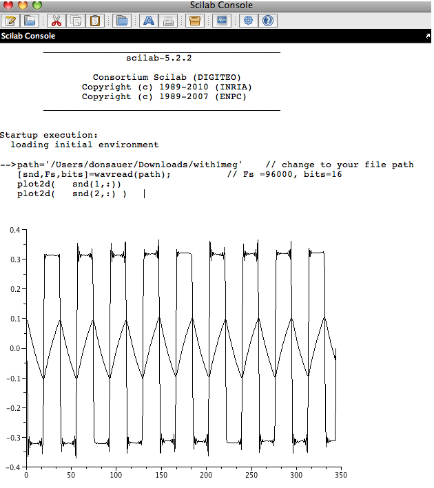
The result should be the following.
=============Copy_Paste_into_Scilab========================
path='/Users/donsauer/Downloads/with1meg' // change to your file path
[snd,Fs,bits]=wavread(path); // Fs =96000, bits=16
plot2d( snd(1,:))
plot2d( snd(2,:) )
=============And_Get_the_Following_Results==================
*=============Find_Your_Gain=====================
==============Copy_Paste_into_Scilab========================
snd(1,10)
snd(1,25)
==============And_Get_the_Following_Results==================
-->snd(1,10)
ans =
- 0.3205261
-->snd(1,25)
ans =
0.3147583
Copy and paste the text above to find actual values.
If +/- Vcc/2 represents +/-31.5% of full scale.
Then +/- full scale is 157% of VCC, or 7.87 if VCC is 5.00 volts.
The actual value for your laptop may vary.
For this actual circuit, some further hardware calibrations were needed.
Adding 1mA to the ICS node produces a change of 1.2volts.
The gain for voltage was really 7.78.
The gain for current for this circuit is then .0066.
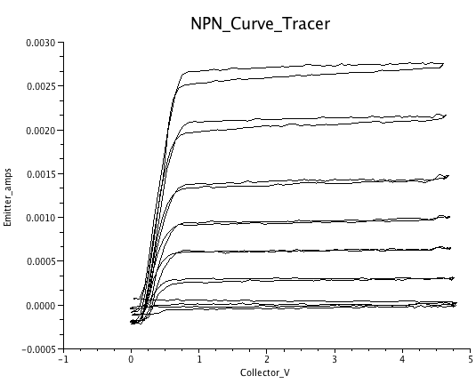
*=============Translate_A_NPN_Curve=====================
Download the captured NPN curve into a known path.
Correct the path of text below before pasting it into a scilab window.
The following will gain scale and offset shift captured waveforms.
An NPN curve tracer graph is displayed in terms of voltages and currents.
Since all signals are AC coupled,
offsets will need to be adjusted to bring the origin close to zero.
============Copy_Paste_into_Scilab========================
path='/Users/donsauer/Downloads/npn.wav' // fix your file path
[snd,Fs,bits]=wavread(path);
[ch,n]=size(snd)
a=get("current_axes");
t=a.title;
t.font_size=4;
plot2d( 7.78*snd(1,1:n-5)+2.6, 0.0066*snd(2,1:n-5) +.8e-3 ) //add gain offset
xtitle("NPN_Curve_Tracer","Collector_V","Emitter_amps");
=============And_Get_the_Following_Results==================
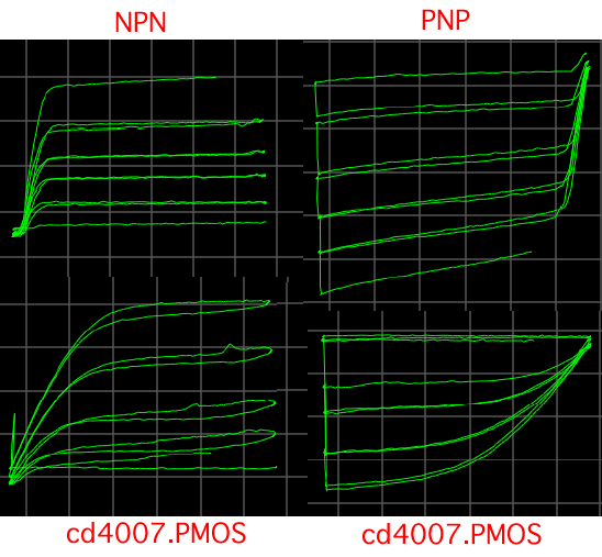
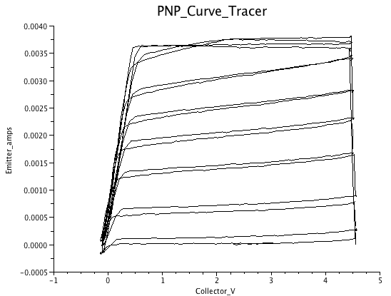
*=============Translate_A_PNP_Curve=====================
Download the captured PNP curve into a known path.
For PNPs, the gain scales can be inverted to resemble an NPN.
============Copy_Paste_into_Scilab========================
path='/Users/donsauer/Downloads/pnp.wav' // fix your file path
[snd,Fs,bits]=wavread(path);
[ch,n]=size(snd)
a=get("current_axes");
t=a.title;
t.font_size=4;
plot2d( -7.78*snd(1,1:n-5)+2,-0.0066*snd(2,1:n-5) +1.65e-3 ) //add gain offset
xtitle("PNP_Curve_Tracer","Collector_V","Emitter_amps");
=============And_Get_the_Following_Results==================
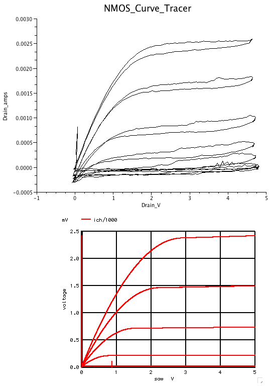
*=============Translate_A_NMOS_Curve=====================
Download the captured NMOS curve into a known path.
A MacSpice simulation for the NMOS in the cd4007 is included.
Simulations and silicon can cross check each other at the same time.
============Copy_Paste_into_Scilab========================
path='/Users/donsauer/Downloads/nmos.wav' // change to your file path
[snd,Fs,bits]=wavread(path);
[ch,n]=size(snd)
a=get("current_axes");
t=a.title;
t.font_size=4;
plot2d( 7.78*snd(1,1:n-5)+2.6, 0.0066*snd(2,1:n-5) +.49e-3 ) //add gain offset
xtitle("NMOS_Curve_Tracer","Drain_V","Drain_amps");
=============And_Get_the_Following_Results==================
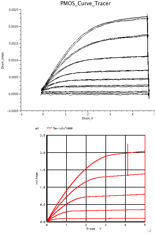
*=============Translate_A_PMOS_Curve=====================
Download the captured PMOS curve into a known path.
A MacSpice simulation for the PMOS in the cd4007 is included.
nmos.wav
NMOS_CURVETRACER.cir
Simulations and silicon can cross check each other at the same time.
============Copy_Paste_into_Scilab========================
path='/Users/donsauer/Downloads/pmos.wav' // change to your file path
[snd,Fs,bits]=wavread(path);
[ch,n]=size(snd)
a=get("current_axes");
t=a.title;
t.font_size=4;
plot2d( -7.78*snd(1,1:n-5)+2.1, -0.0066*snd(2,1:n-5) +.55e-3 ) //add gain offset
xtitle("PMOS_Curve_Tracer","Drain_V","Drain_amps");
=============And_Get_the_Following_Results==================
*=============Other_CurveTracer_Uses=====================
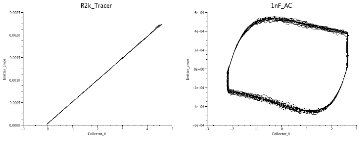
Using clip leads to connect PorN was in hindsight a blessing.
Construct another voltage reference which is half supply,
and have it be able to sink and source current,
and full +/- curve tracing is enabled.
This might come in handy measuring nonlinear resistors.
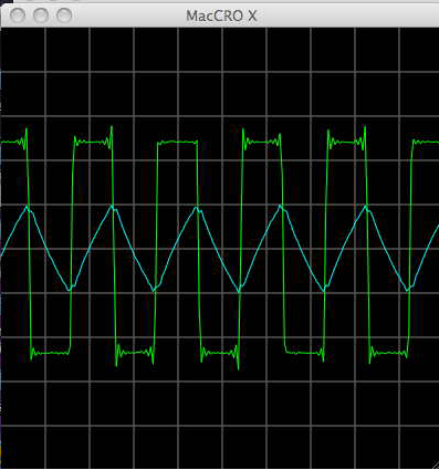
The sweeping voltage is a clipped triangle wave.
Capacitance almost are displayed as a square.
Piezo Electric transducers look like capacitors.
*=============Measure_LEDS=====================
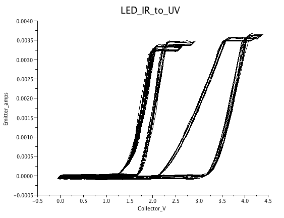
One would expect different LEDs to have different V/I curves.
The IR LED appears to have the lowest voltage and UV the highest.
*=============Investigate_Photo_Devices=====================
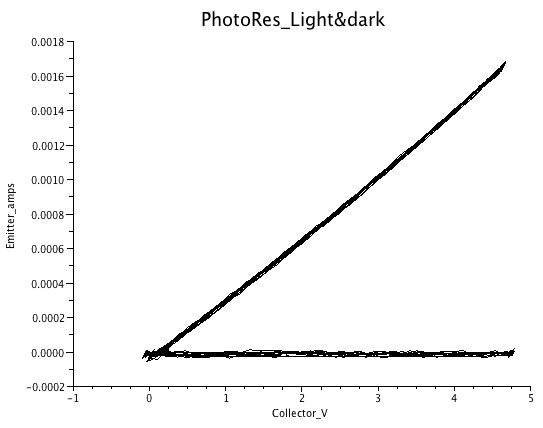
Things like photo resistors are fun to play with.
The MacCRO X application can display the effects of light real time.
The photo resistor is an open in the dark.
*=============Measure_IC_Start_UP=====================
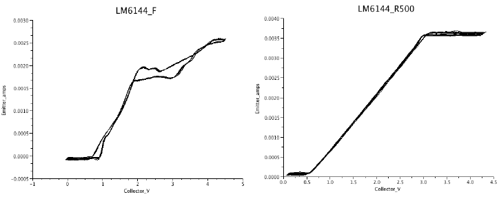
One can see how an IC starts up by looking at supply current.
The LM6144 has a bandgap which starts up at a diode and sat voltage.
The bandgap is designed to turn on everything to be functional,
but in an extremely current limited mode.
This has been called graceful death.
It allows an Op Amp to power down without going crazy.
In the reverse direction, an IC is just a diode.
This curve tracer circuit want some series R when measuring diodes.